Spring 2026 Weekly Updates

2026-03-25

Week 9

Questions
Geocoding with tidygeocoder or arcgisgeocode
Writing functions in R
Creating projects with Quarto
Exploratory data analysis

Questions

What does the “loess” method mean in the [geom_smooth](https://ggplot2.tidyverse.org/reference/geom_smooth.html) function? “loess” is for LOESS (locally estimated scatterplot smoothing) - a local regression method.

Is there a rule of thumb of when to create a function or is it mostly just “you know you need one when you think you do”?
How do I decide when it’s worth turning code into a function instead of just keeping it in-line?
In data science workflows, how do we best balance the Don’t Repeat Yourself principle and the use of existing packages with the educational value of writing algorithms from first principles?

Week 6

Schedule adjustment for 4/1
Reminders
- Exercise 3 due today
- Exercise 4 due Wednesday, 3/11
- Exercise 5 coming soon
- Exercise 1, 2, or 3 questions?
Final Project Timeline
- Project proposal - due Wednesday, 3/25
- Final project presentations - due Monday, 5/4
- Final project repository - due Friday, 5/15
Questions
Recap: Creating and manipulating attributes for spatial data
Lecture: Working with spatial and geometric operations in {sf}
Review two-table verbs with dplyr

Questions

How do you decide the “right” structure for a dataset when it can be organized in more than one tidy way? - Vrinda

Typically, whatever format allows you to efficiently complete the necessary analysis and produce the expected outputs is the “right” structure.

How much does it matter when making the decision on what function to use when smoothing? - Dillon

Check out the smoothr documentation for more details.

You can also use sf::st_simplify() or rmapshaper::ms_simplify() for make less “smooth” lines and polygons.

Which carrier has the worst average delays? Check R for Data Science (2e) - Solutions to Exercises for tips.

nycflights13::flights |>
  group_by(carrier) |>
  summarise(avg_delay = mean(arr_delay, na.rm = TRUE)) |>
  slice_max(order_by = avg_delay, n = 1)

# A tibble: 1 × 2
  carrier avg_delay
  <chr>       <dbl>
1 F9           21.9

Can you disentangle the effects of bad airports vs. bad carriers? (via Solutions Manual: R for Data Science (2e))

nycflights13::flights |>
  group_by(dest, carrier) |>
  summarise(avg_delay = mean(arr_delay, na.rm = TRUE)) |>
  # taking the highest average delay flight at each airport
  slice_max(order_by = avg_delay, n = 1) |>
  ungroup() |>
  # for each airline, summarize the number of airports where it is
  # the most delayed airline
  summarise(n = n(), .by = carrier) |>
  slice_head(n = 5) |>
  arrange(desc(n)) |>
  rename(Carrier = carrier, `Number of Airports` = n) |>
  gt::gt()

Carrier	Number of Airports
EV	42
B6	20
UA	14
AA	6
FL	2

How do you choose when to use st_intersection() vs. st_join() when looking at relationships between layers? - Liam

nc <- st_read(system.file("shape/nc.shp", package = "sf"))

Reading layer `nc' from data source 
  `/Users/bldgspatialdata/Library/R/arm64/4.5/library/sf/shape/nc.shp' 
  using driver `ESRI Shapefile'
Simple feature collection with 100 features and 14 fields
Geometry type: MULTIPOLYGON
Dimension:     XY
Bounding box:  xmin: -84.32385 ymin: 33.88199 xmax: -75.45698 ymax: 36.58965
Geodetic CRS:  NAD27

nc_points <- st_as_sf(st_sample(nc, 250))

st_join(nc_points, nc[1, ])

Simple feature collection with 250 features and 14 fields
Geometry type: POINT
Dimension:     XY
Bounding box:  xmin: -83.79858 ymin: 33.94363 xmax: -75.81023 ymax: 36.55101
Geodetic CRS:  NAD27
First 10 features:
   AREA PERIMETER CNTY_ CNTY_ID NAME FIPS FIPSNO CRESS_ID BIR74 SID74 NWBIR74
1    NA        NA    NA      NA <NA> <NA>     NA       NA    NA    NA      NA
2    NA        NA    NA      NA <NA> <NA>     NA       NA    NA    NA      NA
3    NA        NA    NA      NA <NA> <NA>     NA       NA    NA    NA      NA
4    NA        NA    NA      NA <NA> <NA>     NA       NA    NA    NA      NA
5    NA        NA    NA      NA <NA> <NA>     NA       NA    NA    NA      NA
6    NA        NA    NA      NA <NA> <NA>     NA       NA    NA    NA      NA
7    NA        NA    NA      NA <NA> <NA>     NA       NA    NA    NA      NA
8    NA        NA    NA      NA <NA> <NA>     NA       NA    NA    NA      NA
9    NA        NA    NA      NA <NA> <NA>     NA       NA    NA    NA      NA
10   NA        NA    NA      NA <NA> <NA>     NA       NA    NA    NA      NA
   BIR79 SID79 NWBIR79                          x
1     NA    NA      NA POINT (-80.61342 35.71325)
2     NA    NA      NA POINT (-80.36994 36.23018)
3     NA    NA      NA POINT (-77.25844 35.57634)
4     NA    NA      NA POINT (-82.28387 35.51869)
5     NA    NA      NA POINT (-82.65556 35.36123)
6     NA    NA      NA POINT (-80.26309 35.21218)
7     NA    NA      NA POINT (-78.07407 35.92356)
8     NA    NA      NA POINT (-78.62108 35.53373)
9     NA    NA      NA POINT (-77.27727 36.50931)
10    NA    NA      NA POINT (-79.74154 34.90924)

st_intersection(nc_points, nc[1, ])

Simple feature collection with 3 features and 14 fields
Geometry type: POINT
Dimension:     XY
Bounding box:  xmin: -81.65456 ymin: 36.27143 xmax: -81.41815 ymax: 36.44493
Geodetic CRS:  NAD27
   AREA PERIMETER CNTY_ CNTY_ID NAME  FIPS FIPSNO CRESS_ID BIR74 SID74 NWBIR74
1 0.114     1.442  1825    1825 Ashe 37009  37009        5  1091     1      10
2 0.114     1.442  1825    1825 Ashe 37009  37009        5  1091     1      10
3 0.114     1.442  1825    1825 Ashe 37009  37009        5  1091     1      10
  BIR79 SID79 NWBIR79                          x
1  1364     0      19 POINT (-81.41815 36.27143)
2  1364     0      19 POINT (-81.63161 36.41221)
3  1364     0      19 POINT (-81.65456 36.44493)

Week 5

Reminder
- Exercises 2 due Friday, 2/27
- Exercise 3 due Wednesday, 3/4
Interesting and Difficult Things!
Week 5 Questions
Finish review of Transforming data with {dplyr}
Creating and manipulating attributes for spatial data

Interesting Things

“honestly was just surprised how easy it is to perform geometry operations”
“we can use distance based joins on two datasets that are meaningfully related even when they don’t intersect”

Difficult Things

“learning how to do the same thing in multiple different ways”
“understanding the different binary operators… st_intersects and st_disjoint were intuitive but others like st_covered_by were less clear”
“finding the time to do the readings”

Questions

“Have you ever had to use DE-9IM strings, will I ever have to use them, can they be practically effectively used by people who are not deep into the lore??” - Lauren

“Do unary and binary geometry operations change the input file or allow you to create a unique output file” - Connor

Week 4

Updates and reminders
- Common issues with syntax
- Exercise how-to with Quarto
- Exercises 2 and 3 due Friday, 2/27 and Wednesday 3/4 (links coming soon)
- Office Hours on Friday, 2/20 at 12:00 pm
Week 4 Questions
Finish review of data visualization example with ggplot2
Transforming data with {dplyr}

Questions

When subseting with the [ operator, why do you need a comma and space at the end? e.g. world[world$area_km2 < 10000, ] —Chase

Use ?[ to take a look at the documentation. When using the [ operator to subset a data frame (or an sf object), the first value is the row index and the second is the column index.

# Select second row
us_states[2, ]

Simple feature collection with 1 feature and 6 fields
Geometry type: MULTIPOLYGON
Dimension:     XY
Bounding box:  xmin: -114.8136 ymin: 31.33224 xmax: -109.0452 ymax: 37.00426
Geodetic CRS:  NAD83
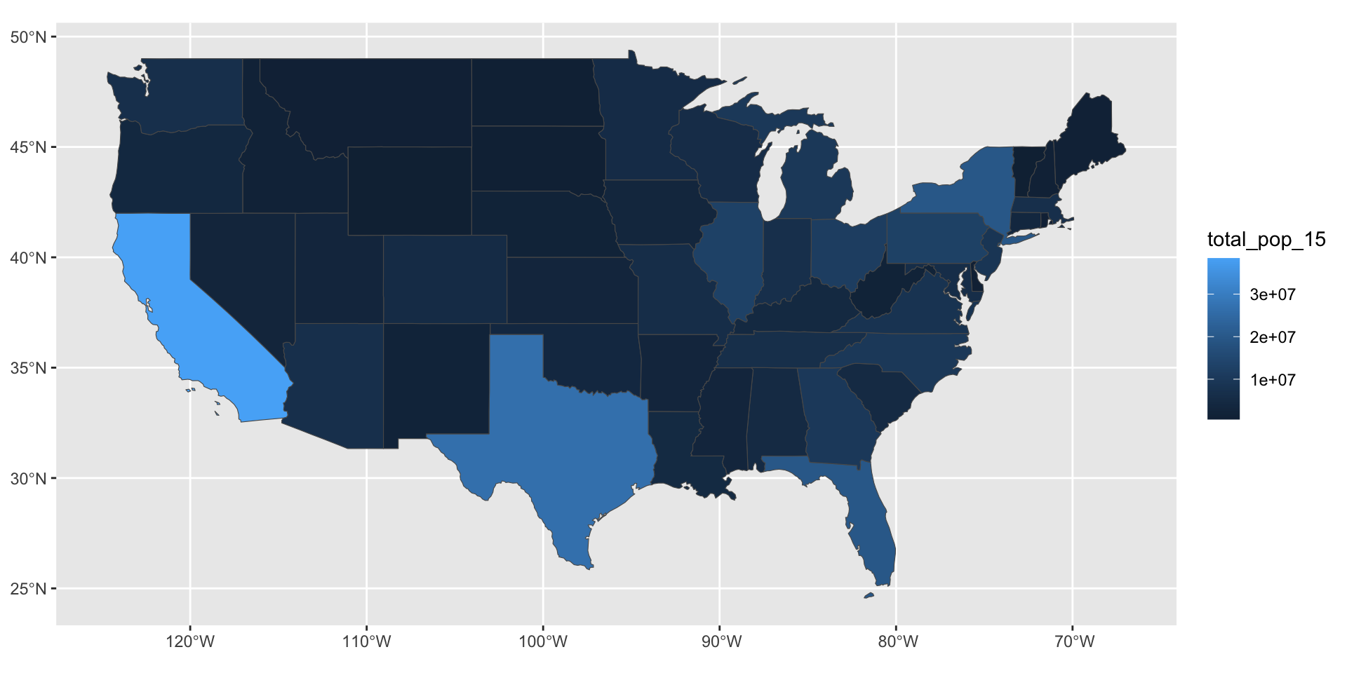
  GEOID    NAME REGION            AREA total_pop_10 total_pop_15
2    04 Arizona   West 295281.3 [km^2]      6246816      6641928
                        geometry
2 MULTIPOLYGON (((-114.7196 3...

# Select second column
us_states[, 2]

Simple feature collection with 49 features and 1 field
Geometry type: MULTIPOLYGON
Dimension:     XY
Bounding box:  xmin: -124.7042 ymin: 24.55868 xmax: -66.9824 ymax: 49.38436
Geodetic CRS:  NAD83
First 10 features:
          NAME                       geometry
1      Alabama MULTIPOLYGON (((-88.20006 3...
2      Arizona MULTIPOLYGON (((-114.7196 3...
3     Colorado MULTIPOLYGON (((-109.0501 4...
4  Connecticut MULTIPOLYGON (((-73.48731 4...
5      Florida MULTIPOLYGON (((-81.81169 2...
6      Georgia MULTIPOLYGON (((-85.60516 3...
7        Idaho MULTIPOLYGON (((-116.916 45...
8      Indiana MULTIPOLYGON (((-87.52404 4...
9       Kansas MULTIPOLYGON (((-102.0517 4...
10   Louisiana MULTIPOLYGON (((-92.01783 2...

Do you always use sf objects when working with spatial data? Or do you switch between spatial and non-spatial formats? —Liam

Yes. Always drop the geometry using sf::st_drop_geometry() if you don’t need it in your output!

Summarising a data frame vs. sf object with bench::mark

storms_sf <- sf::st_as_sf(storms, coords = c("long", "lat"), crs = 4326)

comparison <- bench::mark(
  df = storms |>
    dplyr::summarise(
      mean_wind = mean(wind),
      .by = year
    ),
  sf = storms_sf |>
    dplyr::group_by(year) |>
    dplyr::summarise(
      mean_wind = mean(wind)
    ),
  check = FALSE
)

Error in `ggplot2::autoplot()`:
! The package "ggbeeswarm" is required to use `type = "beeswarm".

Does it matter the order that you specify parameters for a ggplot? —Lauren

Consistent code style improves the readability of your code and reduces risk of errors but ggplot2 supports a flexible approach.

This works…

ggplot(data = us_states) +
  geom_sf(aes(fill = total_pop_15))

…and this works…

ggplot(data = us_states) +
  aes(fill = total_pop_15) +
  geom_sf()

…and this works!

ggplot() +
  geom_sf(data = us_states, aes(fill = total_pop_15))

But… this does not work! Do you know why?

ggplot() +
  geom_sf(us_states, aes(fill = total_pop_15))

Error in `layer_sf()`:
! `mapping` must be created by `aes()`.
✖ You've supplied a <sf> object.

Finish review

Download the example script to review:

usethis::use_github_file(
  repo = "bldgspatialdata/website",
  path = "examples/data-visualization.R"
)

Week 3

Questions

What are some effective ways to familiarize yourself with the language of different packages without rote memorization of their functions? —Brian

Cheatsheets, e.g. RStudio, ggplot2
Community resources, e.g. ggplot2 Theme Elements Reference Sheet
Naming conventions, e.g. geom_<type of geometry to show on plot>

Is there an easy way to plot summary statistics (e.g. mean, min, max)? —Lauren

summary(spData::us_states_df)

    state           median_income_10 median_income_15 poverty_level_10 
 Length:51          Min.   :20019    Min.   :21438    Min.   :  52297  
 Class :character   1st Qu.:23995    1st Qu.:24952    1st Qu.: 204702  
 Mode  :character   Median :25432    Median :26943    Median : 577247  
                    Mean   :26144    Mean   :27500    Mean   : 802304  
                    3rd Qu.:29072    3rd Qu.:30376    3rd Qu.: 822568  
                    Max.   :35264    Max.   :40884    Max.   :4919945  
 poverty_level_15 
 Min.   :  64995  
 1st Qu.: 238146  
 Median : 636947  
 Mean   : 936256  
 3rd Qu.: 961445  
 Max.   :6135142

Is there an easy way to plot summary statistics (e.g. mean, min, max)? —Lauren

skimr::skim(spData::us_states_df)

Data summary
Name	spData::us_states_df
Number of rows	51
Number of columns	5
_______________________
Column type frequency:
character	1
numeric	4
________________________
Group variables	None

Variable type: character

skim_variable	n_missing	complete_rate	min	max	empty	n_unique	whitespace
state	0	1	4	20	0	51	0

Variable type: numeric

skim_variable	complete_rate	mean	sd	p0	p25	p50	p75	p100	hist
median_income_10	1	26143.84	3562.11	20019	23995.0	25432	29072.0	35264	▅▇▃▃▂
median_income_15	1	27500.08	3797.63	21438	24951.5	26943	30375.5	40884	▇▇▅▁▁
poverty_level_10	1	802304.18	949185.01	52297	204702.0	577247	822568.0	4919945	▇▁▁▁▁
poverty_level_15	1	936255.75	1138461.52	64995	238146.0	636947	961445.0	6135142	▇▁▁▁▁

Why are some CRS values NA while some are specific datum (WGS84, etc)? —Nhi

x <- st_point(c(1, 0))

st_crs(x)

Coordinate Reference System: NA

st_crs(spData::us_states)

Coordinate Reference System:
  User input: EPSG:4269 
  wkt:
GEOGCS["NAD83",
    DATUM["North_American_Datum_1983",
        SPHEROID["GRS 1980",6378137,298.257222101,
            AUTHORITY["EPSG","7019"]],
        TOWGS84[0,0,0,0,0,0,0],
        AUTHORITY["EPSG","6269"]],
    PRIMEM["Greenwich",0,
        AUTHORITY["EPSG","8901"]],
    UNIT["degree",0.0174532925199433,
        AUTHORITY["EPSG","9122"]],
    AUTHORITY["EPSG","4269"]]

Why do some of the exercises start with the library function and not have you initially install a library? —Kyle

# install.packages("tidyverse")

What actually is an observation and how is it different than a variable? —Dillon

A variable is something you can measure. An observation is a set of measurements.